What You Lose When You Discretize Your Search Space
Most optimization libraries force you to define your search space as a grid.
Want to tune a learning rate between 0.001 and 1.0? You create a numpy array:
np.linspace(0.001, 1.0, 100). Sounds reasonable. But you just made a decision
that silently costs you performance, and you probably never thought about it.
You chose 100 steps. Why not 50? Or 500? Or 10,000? Every choice is a tradeoff you shouldn’t have to make. This post is about that tradeoff, how much it actually costs, and how to avoid it entirely.
The setup
Let’s run a simple experiment. We take a well-known benchmark function (the Ackley function, shifted so the optimum sits at an awkward location that doesn’t land on any regular grid) and optimize it four times with the exact same optimizer and budget:
- Continuous: the optimizer can pick any float in the range
- Discrete (200 steps): values snapped to a grid of 200 evenly spaced points
- Discrete (50 steps): same idea, coarser grid
- Discrete (10 steps): very coarse
Same optimizer (Particle Swarm), same number of iterations, same random seeds. The only thing that changes is how the search space is defined.
The discretization tax
Here’s what happens:
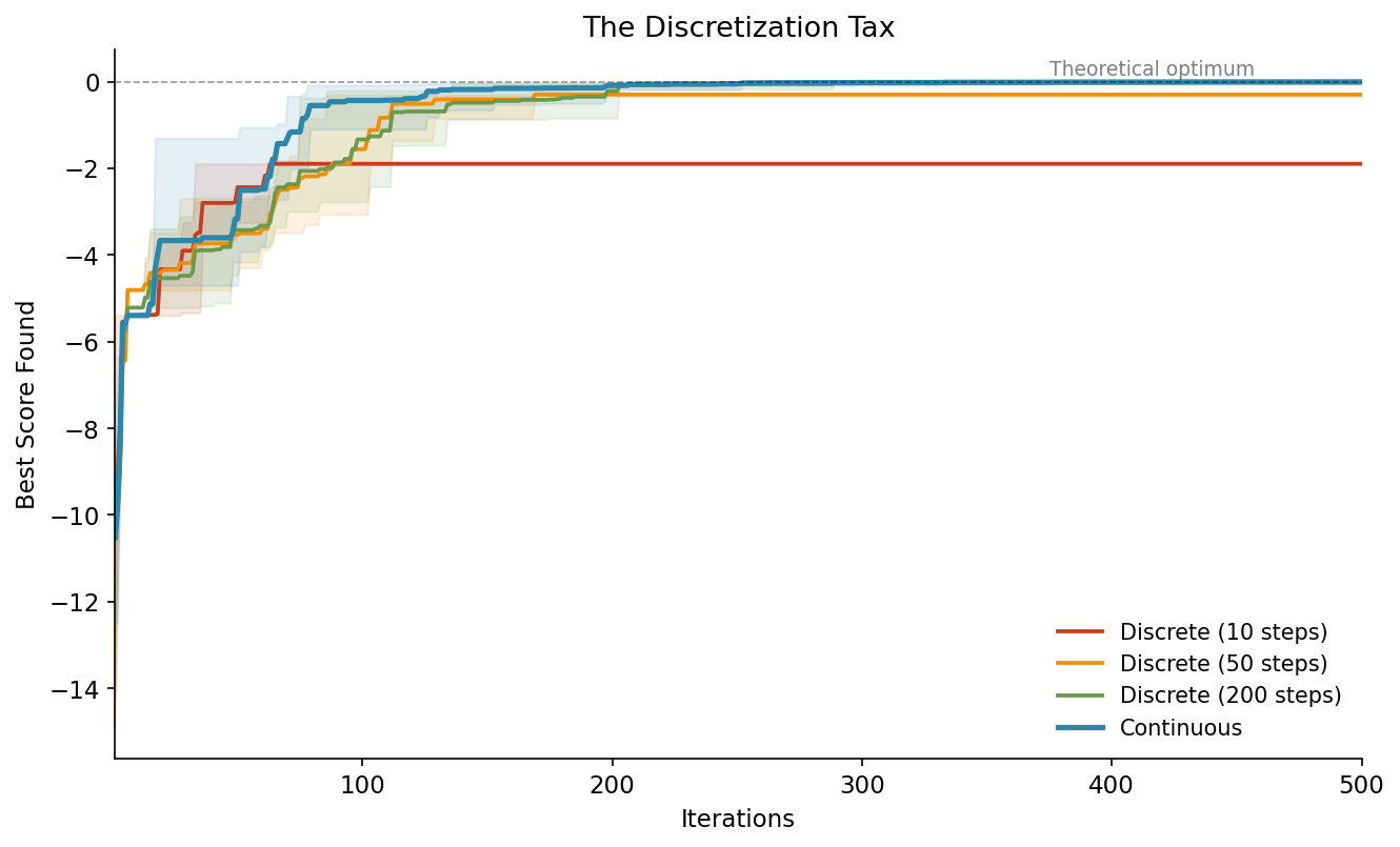
The blue line (continuous) converges faster and ends up closer to the theoretical optimum. The red line (10 steps) hits a ceiling early and stays there. It literally cannot get closer because there’s no grid point near the true optimum.
The shaded bands show the spread across 5 different random seeds. Even in the worst case, continuous beats the best case of coarse discretization.
This is the discretization tax: a hard ceiling on your result that you pay just because of how you defined your search space.
Where the optimizer looks
To see why this happens, let’s look at the actual positions the optimizer evaluates. Here’s the same function, zoomed into the region around the optimum:
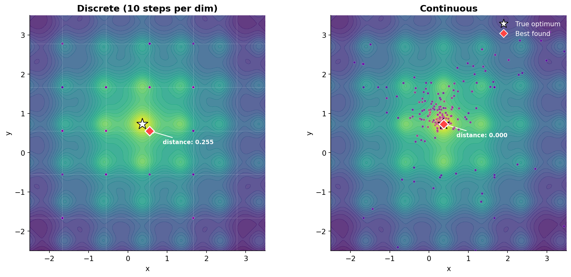
On the left, the optimizer is trapped on a grid. You can see the faint grid lines, and every evaluated point sits exactly on an intersection. The closest grid point to the true optimum (white star) is 0.255 away. That’s not a failure of the optimizer. It’s a hard constraint from the search space definition.
On the right, the optimizer is free to go anywhere. Points cluster tightly around the optimum, and the best found position lands right on top of it (distance: 0.000).
Same optimizer, same budget, same function. The only difference is one line of code in the search space definition.
The resolution dilemma
The obvious fix is: just use more grid points. And yes, that helps. But it creates a new problem:
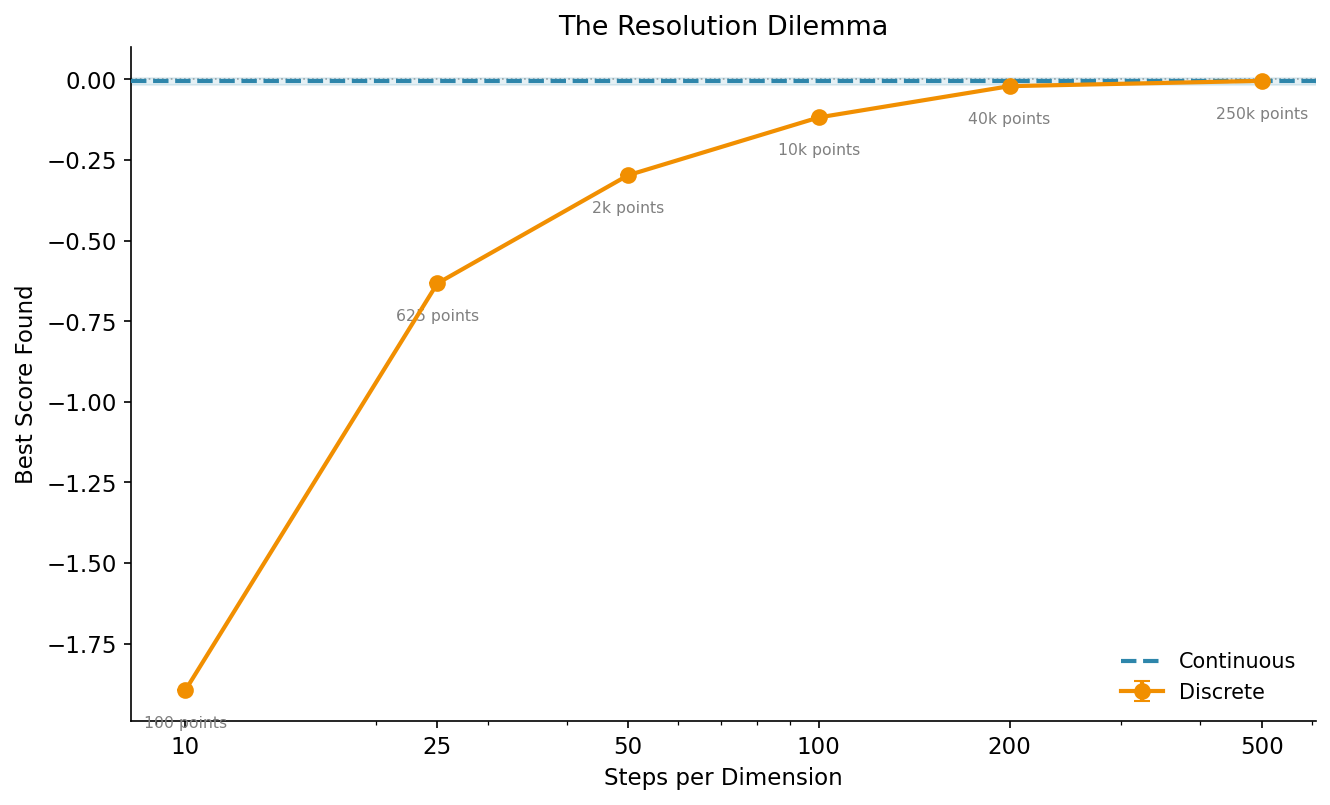
As you increase the number of steps per dimension, the result gets closer to the continuous baseline (dashed blue line). But look at the annotations: the total number of grid points grows quadratically. 10 steps per dimension means 100 points. 500 steps means 250,000 points.
That matters because many optimization algorithms scale with the size of the search space. Larger grids mean more memory, longer initialization, and in some cases slower convergence because the optimizer has more ground to cover.
Continuous search spaces don’t have this problem. There’s no grid, no quadratic blowup, no resolution to choose. The optimizer works directly with float values.
How to use continuous search spaces
If you’re using Gradient-Free-Optimizers, the switch is a one-line change. The library determines the dimension type from the Python data structure you pass in:
import numpy as np
from gradient_free_optimizers import ParticleSwarmOptimizer

search_space = {
    # Discrete: numpy array (the classic way)
    "n_estimators": np.arange(10, 200),

    # Continuous: just a tuple (min, max)
    "learning_rate": (0.0001, 1.0),

    # Categorical: a plain list
    "algorithm": ["adam", "sgd", "rmsprop"],
}

opt = ParticleSwarmOptimizer(search_space)
opt.search(objective_function, n_iter=500)
That’s it. A tuple (min, max) means continuous. A list means categorical. A
numpy array means discrete. No configuration flags, no type annotations. The
data structure is the specification.
And you can mix them freely. A search space with some continuous, some categorical, and some discrete dimensions works out of the box with every optimizer in the library.
When discrete is still the right choice
Continuous search spaces aren’t always better. Some parameters are genuinely discrete:
- Number of layers in a neural network (1, 2, 3, … not 2.7)
- Batch size when you want specific powers of two (32, 64, 128)
- Tree depth in a random forest
For these, numpy arrays or lists are still the right representation. The point isn’t that discrete is bad. The point is that using discrete as a workaround for continuous parameters costs you precision for no reason.
The takeaway
If your parameter is naturally continuous (learning rates, regularization strengths, dropout probabilities, temperature values), define it as continuous. Don’t discretize it just because that’s what the API used to require.
The experiment above shows that even with 200 grid points per dimension, you leave performance on the table. Continuous search spaces remove that ceiling entirely, with zero additional complexity in your code.
All plots in this post are fully reproducible. The experiment uses the Gradient-Free-Optimizers library (v1.10.0+). You can find the complete code on GitHub.